
* 퇴근후딴짓 님의 강의를 참고하였습니다. *
1. 머신러닝
ㅇ기존에는 데이터/규칙을 Rule Base로 결과를 도출하였지만, 머신러닝은 데이터와 결과(해답)을 기반으로 학습을 통해 규칙을 도출하고 머신러닝이 만든 규칙을 기반으로 새로운 데이터를 입력했을 때 결과가 도출되게 됨
- 지도학습 : 분류/회귀 > 빅분기 시험 범위
- 비지도학습
- 강화학습
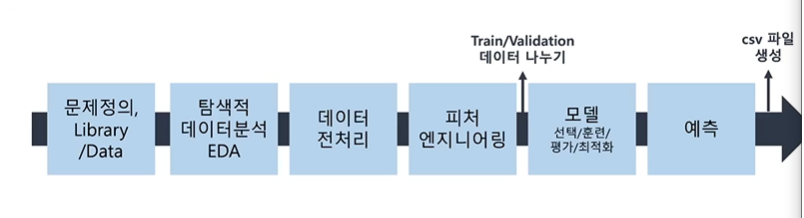
2. 머신러닝 프로세스
ㅇ 문제 정의(Library / Data) > 탐색적 데이터분석(EDA) > 데이터전처리(결측치 : 채우기, 삭제 or 이상치 : 삭제 / 시험문제에서 이상치는 없는 경우가 많음) > 피처 엔지니어링 > Train/Validation(학습용/검증용) 데이터 나누기 > 모델(선택/훈련/평가/최적화) > 예측
3. 시험문제 풀이방법
ㅇ 문제정의, 라이브러리 및 데이터 불러오기
- 분류/회귀 여부
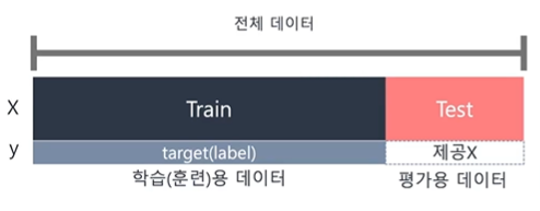
- 데이터set 확인 : 2개(train/test) / 3개(X_train, y_train, X_test)
. X_train/y_train은 훈련용/학습용 데이터이며 X_test는 예측해야 하는 데이터 : X_train(데이터), y_train(해답)로 학습해서 모델을 만들고, X_test 데이터에 대한 결과를 도출
. X는 훈련/학습용 데이터로 독립변수, y는 해답으로 종속변수
- 예측해야 하는 컬럼 및 결과(확률? 0/1?)
- 평가방식
- 최종생성파일(csv파일) 형태
# 라이브러리 및 데이터 불러오기
import pandas as pd

# 데이터set가 3개일 때
X_train = pd.read_csv('X_train.csv')
y_train = pd.read_csv('y_train.csv')
X_test = pd.read_csv('X_test.csv')

# 데이터set이 2개일 때 X_train, X_test라 생각하고 풀기
train = pd.read_csv("train.csv")
test = pd.read_csv("test.csv")
ㅇ 탐색적 데이터분석(EDA)
- 데이터 샘플(head()/tail()), 크기(shape), 컬럼 타입(info()), 결측치(isnull().sum()), 기초통계(describe / describe(include='object'), target(label) 값(y_train['컬럼명'].value_counts()) 확인하기
- 상관관계(corr()), 조건을 만족하는 데이터 개수 확인 (len(변수[조건1&조건2]))
# 데이터 크기
X_train.shape, y_train.shape, X_test.shape

# 데이터 샘플 X_train
X_train.head(3)
y_train.head(3)
X_test.head(3)

# 데이터 타입
X_train.info()

# 결측치
X_train.isnull().sum()
X_test.isnull().sum()

# 기초통계 (object도 확인)
X_train.describe()
X_train.describe(include='object')
X_test.describe(include='object')

# target(label) 값 확인
y_train['gender'].value_counts()
ㅇ 데이터 전처리 : X_train, X_test 2개 모두 처리하기
- 결측치 처리(삭제, 중앙값으로 대체 등) : .fillna(값) / .drop(['컬럼명'], axis=1)
* 삭제 *
. 결측치가 잆는 데이터(행) 전체 삭제 및 확인 : X_train.dropna()
. 특정컬럼에 결측치가 있으면 데이터(행) 삭제 : X_train.dropna(subset=['컬럼', '컬럼2'])
. 결측치가 있는 컬럼(열) 삭제 : X_train.dropna(axis=1)
. 결측치가 있는 특정 컬럼(열) 삭제 : X_train_drop(['컬럼명'], axis=1)
. 중복값 제거 : X_train.drop_duplicates()
* 채우기 *
. 최빈값
m = X_train['workclass'].mode()[0] # 최빈값
X_train['workclass'] = X_train['workclass'].fillna(m)
. 결측값을 새로운 카테고리로 생성
X_train['occupation'] = X_train['occupation'].fillna('X')
- 이상치(IQR) 처리 (! X_test 데이터(행) 삭제는 하면 안됨 !)
(ex) age가 1이상인 데이터만 살림 : X_train = X_train[X_train['age']>0]
- 학습에 불필요한 컬럼 삭제 : train.drop(cols, axis=1), test.drop(cols, axis=1) # cols는 정의 필요
# 결측치처리
X_train = X_train.fillna(0) # 환불금액 0값으로 채움
X_test = X_test.fillna(0)

# id 삭제함 (test의 id값은 csv파일을 생성할 때 필요함으로 옮겨 놓음)
X_train = X_train.drop(['cust_id'], axis=1)
cust_id = X_test.pop('cust_id')

# 타겟커럼 처리
target = y_train['타겟컬럼']
ㅇ 피처 엔지니어링 : X_train, X_test 2개 모두 처리하기 (수치형/범주형 데이터 분리 > 수치형/범주형 데이터 변환 > 변환한 분리 데이터 다시 합치기)
- 수치형/범주형 데이터 분리 : select_dtypes(exclude/include = 'object').copy()
# 수치형 컬럼과 범주형 컬럼 데이터 나누기
n_train = X_train.select_dtypes(exclude='object').copy() # 수치형
n_test = X_test.select_dtypes(exclude='object').copy()

c_train = X_train.select_dtypes(include='object').copy() # 범주형
c_test = X_test.select_dtypes(include='object').copy()

# 데이처 확인
n_train.head()
c_train.head()
- 수치형(int, float) : cols 정의, 함수 불러오기, train데이터 fit_transform, test데이터 transform
. min-max 스케일 : 모든 값을 0과 1 사이로 들어오게 만드는 것
. 표준화 : 평균 0, 표준편차1인 정규분포로 만들기
. 로버스터 스케일링 : 중앙값과 사분위 값 활용, 이상치 영향 최소화 장점
############### MinMaxScaler ###############
from sklearn.preprocessing import MinMaxScaler
cols = ['총구매액', '최대구매액', '환불금액', '내점일수', '내점당구매건수', '주말방문비율', '구매주기']
# cols = X_train.select_dtypes(exclude='object').columns
scaler = MinMaxScaler()
X_train[cols] = scaler.fit_transform(X_train[cols])
X_test[cols] = scaler.transform(X_test[cols])
X_train.head()

############### StandardScaler ###############
from sklearn.preprocessing import StandardScaler
scaler = StandardScaler()
X_train['bmi'] = scaler.fit_transform(X_train[['bmi']])
X_test['bmi'] = scaler.transform(X_test[['bmi']])

############### RobustScaler ###############
from sklearn.preprocessing import RobustScaler
cols = ['총구매액', '최대구매액', '환불금액', '내점일수', '내점당구매건수', '주말방문비율', '구매주기']
scaler = RobustScaler()
display(n_train.head(2))
n_train[cols] = scaler.fit_transform(n_train[cols])
n_test[cols] = scaler.transform(n_test[cols])
display(n_train.head(2))
- 범주형(object) : cols 정의, 함수 불러오기,
. 라벨 인코딩 : 카테고리가 많은 경우
. 원핫 인코딩 : 카테고리가 적은 경우, train/test 데이터프레임 합친 후 인코딩 후 분리하기 get_dummies()
(ex) 데이터 카테고리 : 의류, 디지털, 가전, 디지털, 건강기능
(라벨 인코딩) : 카테고리 1, 2, 3, 2, 4
(원핫 인코딩) : 의류 1 0 0 0 0 / 디지털 0 1 0 1 0 / 가전 0 0 1 0 0 / 건강기능 0 0 0 0 1
########### 라벨인코딩 ###########
# from sklearn.preprocessing import LabelEncoder
# cols = ['주구매상품', '주구매지점']
# cols = X_train.select_dtypes(include='object').columns
# print(cols)

# for col in cols:
#     le = LabelEncoder()
#     X_train[col] = le.fit_transform(X_train[col])
#     X_test[col] = le.transform(X_test[col])

# X_train.head()

from sklearn.preprocessing import LabelEncoder
col = '주구매상품'
le = LabelEncoder()
X_train[col] = le.fit_transform(X_train[col])
X_test[col] = le.transform(X_test[col])

col = '주구매지점'
le = LabelEncoder()
X_train[col] = le.fit_transform(X_train[col])
X_test[col] = le.transform(X_test[col])

X_train.head()


########### 원핫인코딩 ###########
display(c_train.head())
c_train = pd.get_dummies(c_train[cols])
c_test = pd.get_dummies(c_test[cols])
display(c_train.head())
- 데이터 합치기 : concat
. df = pd.concat([X-train, y_train['컬럼명']], axis = 0 or 1) # axis 0은 데이터를 아래로 추가 / 1은 key값 기준으로 컬럼을 추가
- 데이터 분리 : iloc, copy
. X_tr = train.iloc[:, :-1].copy() # 전체데이터 중 마지막컬럼 전까지
. y_tr = train.iloc[:, [0,-1]].copy() # 전체데이터 중 id, 마지막컬럼
# train 데이터에서 범주형 컬럼 정의
cols = list(X_train.columns[X_train.dtypes == object])
print(X_train.shape, X_test.shape)

# train, test 데이터 합치고 원핫인코딩
all_df = pd.concat([X_train, X_test]) # 위 아래로 합침 / 옆으로 붙일 경우 axis=1
all_df = pd.get_dummies(all_df[cols]) # 원핫인코딩 실행

# train, test 데이터 분리
line = int(X_train.shape[0])
X_train = all_df.iloc[:line,:].copy() #처음부터 line까지 잘라내고
X_train
X_test = all_df.iloc[line:,:].copy() #line부터 끝까지
X_test

print(X_train.shape, X_test.shape)
* 수치형/범주형 데이터 나누기 > 수치형은 MinMax스케일링 / 범주형은 라벨인코딩 > 분리해서 변환한 데이터를 X_train, X_test로 다시 합치기
# 수치형 컬럼과 범주형 컬럼 데이터 나누기
n_train = X_train.select_dtypes(exclude='object').copy() # int, float 형
n_test = X_test.select_dtypes(exclude='object').copy()
c_train = X_train.select_dtypes(include='object').copy() # object형
c_test = X_test.select_dtypes(include='object').copy()

# 수치형 - MinMax 스케일링
cols = ['age', 'fnlwgt', 'education.num', 'capital.gain', 'capital.loss', 'hours.per.week']
from sklearn.preprocessing import MinMaxScaler
scaler = MinMaxScaler()
n_train[cols] = scaler.fit_transform(n_train[cols])
n_test[cols] = scaler.transform(n_test[cols])

# 범주형 - 라벨 인코딩
cols = ['workclass', 'education', 'marital.status', 'occupation', 'relationship', 'race', 'sex', 'native.country']
from sklearn.preprocessing import LabelEncoder
le = LabelEncoder()
for col in cols:
    le = LabelEncoder()
    c_train[col] = le.fit_transform(c_train[col])
    c_test[col] = le.transform(c_test[col])

# 분리한 데이터 다시 합침
X_train = pd.concat([n_train, c_train], axis=1)
X_test = pd.concat([n_test, c_test], axis=1)
print(X_train.shape, X_test.shape)
X_train.head()


#### 타겟 컬럼이 비교형(<=50K, >50K)인 경우, 수치형으로 datatype변경
# (y_train['컬럼']!= '<=50K').astype(int)
ㅇ 훈련(Train) / 검증(Validation) 데이터 나누기
# 검증 데이터 분리1
from sklearn.model_selection import train_test_split
X_tr, X_val, y_tr, y_val = train_test_split(X_train,
                                            y_train['gender'], # 타겟컬럼만 선정
                                            test_size=0.2, # 검증용 데이터로 가져갈 비율
                                            random_state=2022) #매번 실행할 때마다 동일하게 분리하기 위해 값 지정
X_tr.shape, X_val.shape, y_tr.shape, y_val.shape


# 검증데이터 분리2
from sklearn.model_selection import train_test_split
X_tr, X_val, y_tr, y_val = train_test_split(train.drop('TravelInsurance', axis=1), # 타겟컬럼 제외한 학습데이터
                                            train['TravelInsurance'], # 타겟컬럼
                                            test_size=0.1,
                                            random_state=1204)
X_tr.shape, X_val.shape, y_tr.shape, y_val.shape
ㅇ 모델 선택/훈련/평가/최적화
(모델) : 모델 불러서 학습(fit)하고, validation 데이터로 예측(predict/ 확률은 predict_proba)하기 // X_tr, y_tr로 모델 학습시키고 X_val 데이터로 예측해서 y_val로 타겟컬럼 예측/확률 등 평가하기
- 분류 : RandomForest, Decision Tree, XGBoost, 로지스틱회귀
- 회귀 : RandomForest, Linear Regression, XGBoost
* 하이퍼파라미터 튜닝
. RandomForestClassifier(n_estimators= 200, 400, 800, 1000 많을수록 속도 느림, max_depth = 3~12, random_state = 2022)
. xgb = XGBClassifier(random_state=2022, max_depth=3~12, n_estimators=100~1000, learning_rate=0.1 .... 0.01)
* n_estimators 올릴 때, learning_rate는 내려야 함
### 분류 ###
############ 랜덤포레스트_분류(RandomForestClassifier) ##############
from sklearn.ensemble import RandomForestClassifier
model = RandomForestClassifier(random_state=2022)
model.fit(X_tr, y_tr)
pred = model.predict_proba(X_val)

# 랜덤포레스트
from sklearn.ensemble import RandomForestClassifier
rf = RandomForestClassifier(n_estimators=400, max_depth=9, random_state=1204 )
rf.fit(X_tr, y_tr)
pred = rf.predict_proba(X_val)[:,1]
# 하이퍼파라미터 튜닝 : max_depth(3~12), n_estimator 100이 기본인데 tree 개수 늘리는 거고 많을 수록 속도는 느림(200, 400, 800, 1000)
# rf = RandomForestClassifier(random_state=2022, max_depth=5, n_estimators=400)

############ 의사결정나무 (DecisionTreeClassifier) ##############
from sklearn.tree import DecisionTreeClassifier
dt = DecisionTreeClassifier()
dt.fit(X_tr[cols], y_tr)
pred=dt.predict_proba(X_val[cols])

############ XGBoost (XGBClassifier) ##############
from xgboost import XGBClassifier
xgb = XGBClassifier()
xgb.fit(X_tr[cols], y_tr)
pred=xgb.predict_proba(X_val[cols]) #확률값 예측
# 하이퍼파라미터 튜닝 : max_depth 기본이 3, n_estimator 기본이 100, learning_rate 기본이 0.1인데 n_estimtor 올릴 때 learning_rate는 내려야함
# xgb = XGBClassifier(random_state=2022, max_depth=5, n_estimators=400, learning_rate=0.02)
# max_depth : 3, 4, 5,.... 12
# n_estimators : 100 ~ 1000 / learning_rate : 0.1 .... 0.01

############ 로지스틱회귀 (LogisticRegression) ##############
from sklearn.linear_model import LogisticRegression
model = LogisticRegression(random_state=2022)
model.fit(X_tr, y_tr) # 학습
pred = model.predict_proba(X_val) # 확률 예측


### 회귀 ###
############ LinearRegression ############
from sklearn.linear_model import LinearRegression
model = LinearRegression()
model.fit(X_tr, y_tr)
pred = model.predict(X_val)

############ 랜덤포레스트_회귀 (RandomForestRegressor) ############
from sklearn.ensemble import RandomForestRegressor
model = RandomForestRegressor()
model.fit(X_tr, y_tr)
pred = model.predict(X_val)

############ xgboost Regressor ############
from xgboost import XGBRegressor
model = XGBRegressor(objective='reg:squarederror')
model.fit(X_tr, y_tr)
pred = model.predict(X_val)
(평가)
- ROC_AUC 평가지표
- rmse
- 정확도/정밀도/재현율/F1
############## roc_auc_score ###############
from sklearn.metrics import roc_auc_score
pred = model.predict_proba(X_val) # 0일때 확률, 1일때 확률 2개값 반환
print(roc_auc_score(y_val, pred[:,1])) #1일때 확률

############## rmse ###############
# 평가 수식
from sklearn.metrics import mean_squared_error
import numpy as np
def rmse(y_test, pred):
    return np.sqrt(mean_squared_error(y_test, pred))
# rmse 값 확인
rmse(np.exp(y_val), np.exp(pred))

############## 정확도/정밀도/재현율/F1 ###############
from sklearn.metrics import accuracy_score, precision_score, recall_score, f1_score, roc_auc_score
# 정확도
print(accuracy_score(y_val, pred))
# 정밀도
print(precision_score(y_val, pred))
# 재현율 (민감도)
print(recall_score(y_val, pred))
# F1
print(f1_score(y_val, pred))


############### 평가지표(회귀) ###############
# MAE : 실제값과 예측값 차이를 절대값으로 변환해 평균한 것
# MSE : 실제값과 예측값 차이를 제곱해 평균한 것
# RMSE : MSE에 루트를 씌운 것
# R2 Score : 회귀 모델의 설명력
# RMSLE : 예측값이 실제값보다 작을 때 더 큰 패널티 부여
# MAPE : MAE를 퍼센트로 표시
# R2가 높을 수록, MAE/MSE/RMSE는 낮을 수록 좋은 모델

import numpy as np
from sklearn.metrics import r2_score, mean_absolute_error, mean_squared_error #sklearn에서 제공하는 것
def rmse(y_test, y_pred): #RMSE
    return np.sqrt(mean_squared_error(y_test, y_pred))

def rmsle(y_test, y_pred): #RMSLE
    return np.sqrt(np.mean(np.power(np.log1p(y_test) - np.log1p(y_pred), 2)))

def mape(y_test, y_pred): #MAPE
    return np.mean(np.abs((y_test - y_pred) / y_test)) * 100
ㅇ X_test로 예측 및 최종 파일 제출
- 위에서 만든 모델 중 가장 높은 평가를 받은 모델(피처엔지니어링 변경 / 하이퍼파라미터 조정 / 모델 변경 등)로 X_test 데이터를 활용해 예측
# X_test 데이터로 정답 예측(3개 데이터 set)
pred = model.predict_proba(X_test)
pred

# 데이터 프레임 만들기
submit = pd.DataFrame(
            {
                'cust_id':cust_id,
                'gender':pred[:,1]
            }
        )

# 샘플 데이터 확인
submit.head()

# csv 파일생성
submit.to_csv("000111.csv", index=False)

# csv 파일확인
pd.read_csv("000111.csv")


# test 데이터로 정답 예측(2개 데이터 set)
pred = rf.predict_proba(test)[:,1]
# csv 파일생성
pd.DataFrame({
              'index':test.index,
              'y_prd': pred
}
).to_csv('0000.csv', index=False)
2023.06.12 - [자격증공부/빅데이터분석기사] - [빅데이터분석기사][작업형1] 판다스 문법 활용 요약
[빅데이터분석기사][작업형1] 판다스 문법 활용 요약
1. 라이브러리 및 데이터 읽어오기 ㅇ 컬럼명 확인할 수 있도록 세팅하기 import pandas as pd df = pd.read_csv('ㅇㅇㅇㅇ.csv') pd.set_option('display.max_columns', None) #컬럼명 전부 확인할 수 있도록 셋팅하기 2.
inform.workhyo.com
2023.06.12 - [자격증공부/빅데이터분석기사] - [빅데이터분석기사][작업형3] 가설검정 이론 및 프로세스(정리)
[빅데이터분석기사][작업형3] 가설검정 이론 및 프로세스(정리)
* 퇴근후딴짓 님의 강의를 참고하였습니다. * 1. 모집단과 표본 ㅇ 모집단 : 집단 전체 ㅇ 표본 : 모집단을 대표하는 집합 2. 가설검정 ㅇ 모집단에 대한 가설이 적합한지 추출한 표본데이터로부터
inform.workhyo.com
'자격증공부 > 빅데이터분석기사' 카테고리의 다른 글
| [빅데이터분석기사] 작업형3 가설검정 이론 및 프로세스 (0) | 2023.06.12 |
|---|---|
| [빅데이터분석기사] 작업형1 판다스 문법 활용 요약 (0) | 2023.06.12 |
| [빅데이터분석기사] 작업형2 문제유형 (분류) (0) | 2023.06.12 |
| [빅데이터분석기사] 작업형2 기출문제 3회 (분류) (0) | 2023.06.11 |
| [빅데이터분석기사] 작업형2 기출문제 2회 (분류) (0) | 2023.06.10 |


